Andrés Marafioti, leading the multimodal research team at HuggingFace, wrote about a carefully curated, open-source database of annotated images: FineVision. The goal is to contribute to the Vision Language Model (VLM) community. What’s a VLM? Like an LLM, but it understands images too : i.e., a multimodal model. This made me curious, and I used this database to dabble into the world of multimodality locally. This might be the first in a family of posts exploring this.

First we will take a look at CLIP, one of the early image+text efforts by OpenAI. Then we will dive into a way to detect duplicate content with SSCD. Then we will see how this algorithm can be used to analyze dataset contamination in the context of the FineVision paper, making use of the FAISS library to search these carefully crafted and useful representations.

Interaction with FineVision

Example of one subset of data, and its config dictionary :

ddict = load_dataset("HuggingFaceM4/FineVision", name="chartqa")  
print(ddict)
## --- result ---     
DatasetDict({
    train: Dataset({
        features: ['images', 'texts', 'source', 'relevance_ratings', 'relevance_min', 'image_correspondence_ratings', 'image_correspondence_min', 'visual_dependency_ratings', 'visual_dependency_min', 'formatting_ratings', 'formatting_min'],
        num_rows: 18265
    })
})

There is one split, train, and there are images and texts columns, which are the pairs of figures/captions, in a nutshell. You can see there are also a lot of features useful for quality checks. Ratings and *_min come in pairs : the rating is a list of scores (from 1 the worst to 5 the best), and *_min is the minimum per quality feature. Per the FineVision paper, these were evaluated with LLM/VLM as a judge (“Qwen3-32B for text-only criteria and Qwen2.5VL-32B-Instruct for image-conditioned criteria, served locally via vLLM”). Relevance is how well the answer responds to the question, formatting is the formatting quality of the text, visual dependency is how much the question needs visual info to be answered, and image correspondence is how well the image supports answering the question.

A tentative way to filter on them if you wish:

def pass_quality(ex, min_vd=4, min_ic=3, min_rel=4, min_fmt=3):
	"""
	Uses the dataset's features to add a quality threshold for taking
	rows of samples into account.
	"""
	ok = True
	if "visual_dependency_min" in ex: ok &= ex["visual_dependency_min"] >= min_vd
	if "image_correspondence_min" in ex: ok &= ex["image_correspondence_min"] >= min_ic
	if "relevance_min" in ex: ok &= ex["relevance_min"] >= min_rel
	if "formatting_min" in ex: ok &= ex["formatting_min"] >= min_fmt
	return ok

FineVision’s paper, however, says that these simple prompt-based metrics are not so useful for better training, in contrast to what some other literature shows with other, better metrics. They are handy for quick triage, but do not guarantee better training.

CLIP, a multimodal joint vision and language model from OpenAI

CLIP, or Contrastive Language-Image Pre-training, is a 2021 effort to combine training over image features and text features, learning over pairs of text and captions. This, similarly to the GPT models, is able to then be used for a variety of tasks, without having to specifically train for features or classes (as classical models did). That is why embedding FineVision with it help me search the dataset semantically, maybe check clusters, etc. We will try it in that section, and show you the results.

I note in passing some interesting considerations about the datasets mentioned in the CLIP paper here; I’ve added a bit of information on ImageNet and FineVision, which helps put this dataset into perspective within its context :

Dataset	Raw size	Labeling / metadata quality	Filtering applied	Post-filter size	Notes (from the CLIP paper)
MS-COCO (Lin et al., 2014)	~100,000 training photos	High-quality, crowd-labeled	-	-	Considered small by modern standards
Visual Genome (Krishna et al., 2017)	~100,000 training photos	High-quality, crowd-labeled	-	-	Also small by modern standards
ImageNet (ILSVRC-2012 / ImageNet-1K)	1,281,167 train; 50,000 val; 100,000 test	Curated labels over 1,000 classes	-	-	Canonical large-scale classification set. (image-net.org)
YFCC100M (Thomée et al., 2016)	100,000,000 photos	Sparse / noisy metadata	Kept only images with natural-language titles/descriptions in English	15,000,000	~6× reduction; ends up roughly ImageNet-scale
FineVision (2025)	24,000,000 samples	Unified from >200 sources; curated and audited	Heavy de-dup + benchmark de-contamination; schema unification	24,000,000	~17M images, 89M QA turns, ~10B answer tokens

Embedding with CLIP

from typing import List
import faiss, torch
from PIL import Image
import numpy as np
from transformers import AutoProcessor, CLIPModel

CLIP_ID = "openai/clip-vit-base-patch32"
_device = "cuda" if torch.cuda.is_available() else "cpu"
clip = CLIPModel.from_pretrained(CLIP_ID).to(_device).eval()
clip_proc = AutoProcessor.from_pretrained(CLIP_ID)
print("proj dim:", clip.config.projection_dim)  # 512

@torch.inference_mode()
def clip_text_embed(texts: List[str], device=_device) -> np.ndarray:
    """Text embedding with CLIP model."""
    inp = clip_proc(text=texts, return_tensors="pt", padding=True, truncation=True).to(device)
    v = clip.get_text_features(**inp).detach().cpu().numpy().astype("float32")
    faiss.normalize_L2(v)
    return v

@torch.inference_mode()
def clip_image_embed(pil_images: List[Image.Image], device=_device) -> np.ndarray:
    """PIL images embedding with CLIP model."""
    inp = clip_proc(images=pil_images, return_tensors="pt").to(device)
    v = clip.get_image_features(**inp).detach().cpu().numpy().astype("float32")
    faiss.normalize_L2(v)
    return v

inference_mode and detach are pytorch’s autograd related inference-time optimization, that you have already seen in the QLoRA blog post. clip_proc preprocesses (tokenizes and pads), clip and its subsequent methods encodes via the CLIP text encoder.

Same for images, except that the preprocessing crops, resizes and normalizes images. Both return a (N, D) tensor where N is the number of text and images processed and D is the projection dimension of CLIP’s shared embedding space that can be read with clip.config.projection_dim (512 for the precise model I loaded). Images and texts are projected into the same embedding space of dimension D, and scalar product in this space reflects image/text correspondence.

SSCD, a representation useful to detect copies

In the FineVision paper, they check for train/test samples contamination by using what they call SSCD embeddings. That made me curious and I went and checked the paper, and tried to reproduce their contamination figures. I will explain and show you all this in this section. Finding out whether an image posted on the web is similar to another, for a given website, helps moderate content automatically. That is at least what the SSCD paper tells us. The SSCD method, for self-supervised descriptor for image copy detection, describes how to build such a duplicate detector.

A Convolutional Neural Network (CNN) learns image features and performs tasks on images. SSCD starts with such a CNN (which transforms an image into C learned features maps, like "does it look like a face"-map) and collapses the last layer into a representation vector (via averaging over each feature map with a Generalized Mean or GeM pooling layer - which is a generalization of GAP, global average pooling, i.e., a simple average over each feature map).

from PIL import Image
import numpy as np
from huggingface_hub import snapshot_download
from transformers import pipeline

REPO_ID = "m3/sscd-copy-detection"
snapshot_download(repo_id=REPO_ID)
sscd = pipeline("sscd-copy-detection", model=REPO_ID, device=0)

def sscd_embed(img: Image.Image, size: int = 288) -> np.ndarray:
    vec = sscd(img.convert("RGB"), do_resize=True, size=size)
    vec = np.asarray(vec, dtype="float32")
    vec /= (np.linalg.norm(vec) + 1e-9)
    return vec
img1 = Image.open("a.jpg")
img2 = Image.open("b.jpg")
v1 = sscd_embed(img1)          
v2 = sscd_embed(img2)       
cosine = float(np.dot(v1, v2))  
print("cosine similarity:", cosine)

def sscd_embed_many(images, size: int = 288, batch_size: int = 128) -> np.ndarray:
    outs = sscd(images=[im.convert("RGB") for im in images],
                do_resize=True, size=size, batch_size=batch_size)
    if isinstance(outs, list):
        outs = np.stack([np.asarray(x) for x in outs], axis=0)
    outs = outs.astype("float32", copy=False)
    outs /= (np.linalg.norm(outs, axis=1, keepdims=True) + 1e-9)  
    return outs 

imgs = [Image.open(p) for p in ["a.jpg", "b.jpg", "c.jpg"]]
V = sscd_embed_many(imgs)  

If you want to know more you can read the technique’s paper, linked to at the end of this post.

FAISS, a vector search library by Meta

After embedding the FineVision images and associated texts with the above algorithms, I stored them in FAISS for optimized similarity search.

import faiss, numpy as np
d = V.shape[1]
index = faiss.IndexFlatIP(d) # cosine if inputs are L2-normalized
index.add(V)
D, I = index.search(V[0:1], k=3)
print("top-3 indices:", I[0], "scores:", D[0])

Results and queries

Below you can witness the result of the transformation of these images and texts into the different embedding spaces, and see on a 2-D projection with UMAP how “close” dataset samples are to each other in that space.

Here is the UMAP plot of the text embeddings of the question/answer pairs:

Here is the UMAP plot of the SSCD embeddings of images : Here is the UMAP plot of the CLIP embeddings :

Let us use the SSCD embeddings to look for duplicates in our small samples of the FineVision dataset. We make use of this function, that looks into a FAISS index for all embedded images within a similarity radius so that their similarity $\cos(x_i, x_j) \ge \tau$.

def find_near_duplicates_range(index: faiss.Index, mat: np.ndarray, tau=0.92, batch=100):
    """
    Return list of (i, j, cos) with i < j and cos >= tau using FAISS range_search.
    Assumes mat is L2-normalized and index is IP-based.
    """
    pairs = []
    N = mat.shape[0]
    for start in range(0, N, batch):
        xq = mat[start:start+batch]
        lims, D, I = index.range_search(xq, tau)
        # For each query row r, neighbours are I[lims[r]:lims[r+1]], I are all neighbours indices concatenated, D are all neigbours scores concatenated (see explanation below)
        for r in range(len(xq)):
            a = start + r
            i0, i1 = lims[r], lims[r+1]
            for idx, dist in zip(I[i0:i1], D[i0:i1]):
                b = int(idx)
                if b <= a:  # skip self and reverse duplicates
                    continue
                pairs.append((a, b, float(dist)))
    # Sort most similar first
    pairs.sort(key=lambda t: -t[2])
    return pairs

To better understand how range_search (and the above function) works, an example : Suppose a batch has 3 queries (len(xq)=3) and FAISS returns lims = [0, 2, 5, 6], I = [7, 12, 3,8,10, 4], D = [.97,.94, .96,.93,.92, .95]. It means that for r=0 : neighbours at I[0:2] = [7,12] with scores [.97,.94], for r=1 : neighbours at I[2:5] = [3,8,10] with scores [.96,.93,.92] and query r=2 : neighbours at I[5:6] = [4] with score [.95]. 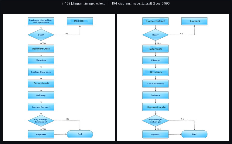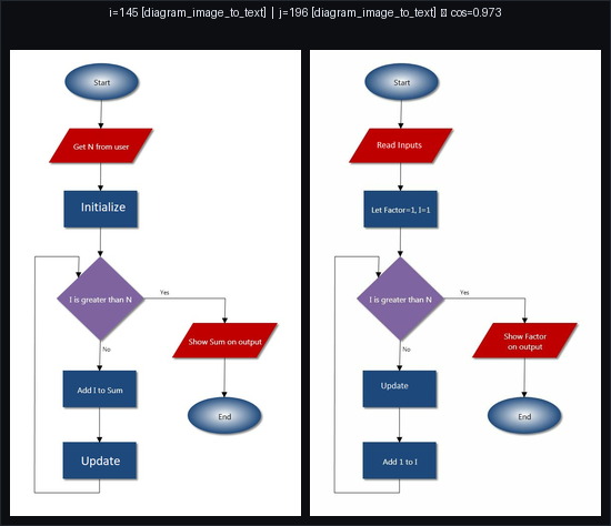Here are my top two examples of duplicates : indeed, it seems these are recycled diagrams.

Doing the same exercise with the CLIP embeddings, I find fewer examples, and there are clear false positives, for example this pair, with a similarity score of 0.975 with CLIP but 0.665 with SSCD. These are small, qualitative examples to build intuition. CLIP is optimized for text–image alignment and SSCD is built for image–image copy detection, so it’s expected to be better for near-duplicates.

For SSCD, I found τ=0.93 a nice qualitative threshold on this subset; raise τ to reduce false positives.

Conclusion, for now

I hope I have given you some taste of what it is like working with FineVision and trying to fetch duplicates and contamination from a dataset. It has helped me brush off some rust on CNNs and learn more about SOTA algorithms and the research in the VLM space. I feel there is a lot more to explore still. I will keep learning on the subject and share insights with you. I might come back to image/text dual datasets very soon, stay tuned!

Useful links

• Learning Transferable Visual Models From Natural Language Supervision
• Faiss library wiki
• A Self-Supervised Descriptor for Image Copy Detection
• FineVision: Open Data Is All You Need
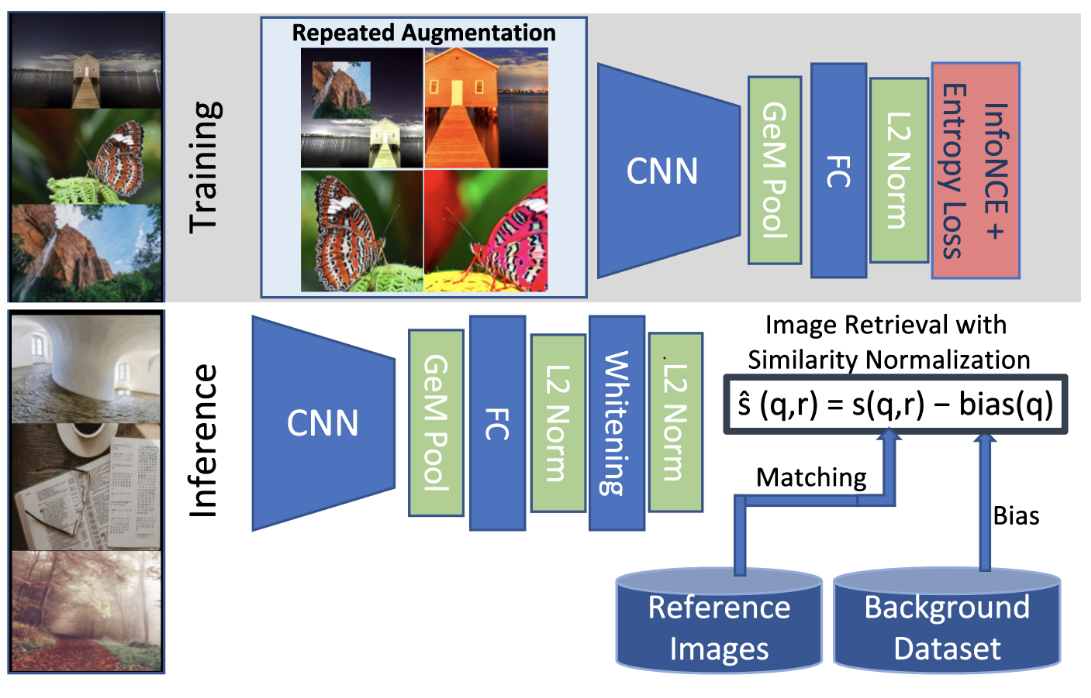
• Fine-tuning CNN Image Retrieval with No Human Annotation
• A Simple Framework for Contrastive Learning of Visual Representations
• ImageNet website
• The CLIP model on HuggingFace
• CLIP transformers docs
• UMAP: Uniform Manifold Approximation and Projection for Dimension Reduction
• How UMAP works
• Benchmark for approximate nearest-neighbour search